@SanPen: do you have an idea why HELM fails here, even though it is supposed to be great for ill-conditioned systems? I tried to do debug into the HELM, but I know to little about the method to be able to check it…
After looking at the 11 bus iwamoto system, it was compiled from this very old paper by hand from the Ybus matrix: https://ieeexplore.ieee.org/document/4111178. So it is very possible that there was a mistake in the conversion, and the system really doesn’t have a solution. Does anyone know of a data set with an ill-conditioned network in a more user friendly format?
#edit: I looked at the iwamoto system some more, and I don’t think we can rely on this network. The original paper does not give units for the admittance matrix (probably per unit, but who knows?) and also defines the power in per unit without giving the base power. Signs for the power (load/generation) are also not given. Its simply not possible to reliably compile the network from the given information.
Further discussion on the mailing list here (for some reason the original post seems to be missing).
And some references below (seeing I posted them to the mailing list). The Wikipedia article is also worth reading.
References
Trias, Antonio (July 2012). The holomorphic embedding load flow method. 2012 IEEE Power and Energy Society General Meeting. New Jersey, USA: IEEE. doi:10.1109/PESGM.2012.6344759.
From what I can see a proper model of that 11-bus grid was not published, but rather the Ybus matrix directly… I observe that Ybus has no symmetry (not even close to symmetry) therefore I’d spend no time with this “grid” since I believe it was created to be non-solvable.
Well according to the paper it was created to be solvable, but difficult to solve. To test the superior convergence behaviour of HELM, we obviously need a network that is difficult to solve. Do you know of any ill-conditioned systems that NR might struggle with?
I can tell you right away that that grid is not only difficult to solve, it is probably impossible to solve.
A simple way to make it hard for NR is to set the specified voltage of some generators high (like 1.12) and others low (like 0.92). There NR will have a hard time solving the voltages since those are not very similar. On the other hand, HELM should work.
Something else that we must bear in mind is that any numerical method has boundaries. Helm included. The HELM convergence properties are supposed to be better but not infinite. Therefore a Y matrix without a symmetrical structure is not solvable by matrix methods. Maybe it is by BFS methods, but those are terrible is meshed grids anyway.
The following paper has the “11 Bus Iwamoto System” branch data (not only the admittance matrix). The authors didn’t detail their reversal engineering process but I remember that their data produce a good approximation of the original admittance matrix (I was introduced to this “11 Bus Iwamoto System” while I was searching for my undergraduate final project a couple years ago).
To be more precise, my undergraduate final project was also about holomorphic embedding load flow. My memory can be fooling me, but I’m almost sure that HELM and NR are both capable of solving this system considering a tolerance about 0.1 MW. I will try to find my stuff back and post it here.
I am Josep Fanals and I think I gave some piece of work worth-sharing.
When it comes to ill-conditioned systems, as stated by Trias, the Padé-Weierstrass method is meant to improve the precision of the solution. I have successfully implemented it and it seems to be the ultimate tool to fight against unacceptable mismatches.
For instance, in the paper mentioned by Zalnd, when all taps become 1 and the loading factor is 0.695, the solution obtained in GridCal yields a minimum error of about 10^{-6} pu (using the Levenberg-Marquardt method). With the basic HELM method the mismatch gets close to 10^{-3} or 10^{-4} at best.
However, the P-W grabs the solution given by the basic HELM and improves the mismatch up to 10^{-11} without much trouble.
I am open to share the code with you if there is interest in the matter.
Iwamoto’s Newton-Raphson: 2nd Taylor approximation (kind of)
LM: Levenberg-Marquardt
HELM: The implicit HELM formulation from Josep and myself
LACPF: Linear AC power flow (it’s linear, it always converges)
DC: Linear so-called “DC” power flow (it’s linear, it always converges)
The lowest error comes from the LM method.
An interesting fact is that if we lower the precision demand to 0.01, NR provides an ok solution, which is clearly a point of improvement in the divergence detector within NR.
With the original tap values I got an initial error of 0.125 MW. Quite similar.
Once I applied the Padé-Weierstrass (P-W) method, the solution did not improve by a lot… At most, it yielded a mismatch of about 0.056 MW. All that considering a loading factor of 0.99194 and depth of 56 coefficients in both the basic HELM and the P-W. The s_0 vector was: [0.3, 0.33, 1].
What shocked me the most was the fact that the elements of the s_0 vector did not approach 1. Instead, when I chose the criteria of using the s_0 values such that the Padé approximants converged up to the desired tolerance, they got closer and closer to 0.
@Zalnd I am curious to know what your s_0 vector was like and how many coefficients you selected.
First of all, allow me to correct the load factor and the maximum error obtained with Padé-Weierstrass. They are 0.99183 and 9.67e-05 MW. That’s the result after some changes in the code.
My basic HELM implementation follows the canonical embedding but my Padé-Weierstrass implementation follows an embedding that expands the Taylor Series from a true operation point and the s-variable works as a load factor. In order to obtain the previous result, I started solving the system considering a load factor of 0.1. From that solution my Padé-Weierstrass implementation finished the job. Three transformations were necessary to obtain the previous result considering 1e-4 MW (1e-6 pu) the maximum error allowed.
All formulations are experimental at some point. @jfbhere has like 10 different formulations.
When I started, my formulations were also experimental, and yet I published the code.
If you’re preparing a paper and are afraid of someone copying, understand that I am an “industry guy”, and my goal in life is not to publish, so I could not care less about that. My goal here is to understand this and maybe benefit from the side effects.
It’s up to you but I encourage you to share your work, because open science improves it’s quality. And that is what this site is about.
If I was worried about publishing it would be prudent not to say even the idea (nothing personal).
Anyway, I fell into the openmod forum searching about open code load flow programs because I do have some things I would like to share. The best of all is that GridCal was coded using Python, a language I’m not familiar with. So, the idea is to force myself to learn it in the process.
About the helm formulation in GridCal, I didn’t understand why the slack equation was implicitly embedded. I mean, I don’t see how your formulation can benefit from that. In the canonical formulation, embedding the slack bus allows to enforce 1 pu as the s=0 solution in all buses. That doesn’t happen in your formulation. Just for curiosity I ran some tests without embedding the slack bus. I also implemented a formulation that eliminates Q from the linear equation system. Surprisingly, that formulation is slower than the original because leads to more complex convolutions. Anyway, you can check the following .py.
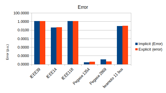
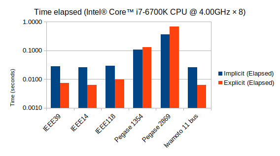
I am particularly happy that you sent the code already in GridCal compatible syntax, so I didn’t have to make any change to make this run. The tests using the code you provided are the following:
Implicit: Implicit slack method (by Josep) Explicit: Explicit slack method as provided by Andre
I don’t see the advertised results for the Iwamoto Grid (1e-6 p.u.).
The explicit method is indeed faster for some grids, but slower for others. In general the precision is comparable (if not the same)
I also noticed that the U[0] coefficients in the formulation provided are not 1+0j either. I understand that the Padè-Weirtrass formulation by @jfb addresses that by separating the admittances in symmetric, asymmetric and shunt.
Actually, in that first test both implementations was born from Josep Implicit Slack formulation. I was trying to address two points: “to embed, or not to embed” the slack voltage equation and to eliminate the Q from the system of linear equations.
In order to avoid confusion, I put back the original formulation in the file. Now there are three formulations:
(a) (…)_josep: Implicit Slack with embedded voltage slack equation (linear system of equations has Q as variable and needs to calculate the coefficients from inverse voltage functions)
(b) (…)_josep_without_slk_emb: Implicit Slack without embedding voltage slack equation (linear system of equations has Q as variable and needs to calculate the coefficients from inverse voltage functions)
(c ) (…)_andre: Implicit Slack without embedding voltage slack equation (Q was eliminated from the linear system of equations and there is no need to calculate inverse voltage functions)
You can check that (b) and (c ) are “essentially” the same in the sense that represent the same set of algebraic voltage functions (check the Taylor series coefficients).
It seems that you are interested about the canonical embedding (the basic helm formulation I also talked about). I supposed that you already have tried it. But I can put that one on the list, no problem.
And finally, about the PW technique on the “taylor-series-expansion-from-a-true-load-flow-solution” embedding (the formulation that naturally corresponds to a PV-Curve). As I stated before, making it available in GridCal it’s also on my plans. But that first test has nothing to do with it.
Having tested a genetic algorithm for solving the OPF I can confirm that it is suboptimal. Even the traditional linear programming yielded better results in the IEEE14 bus.
Back to the holomorphic embedding, I found some interesting results while solving the 11 bus system. First, both the basic NR and the Iwamoto’s NR the voltage values belonged to the negative branch of the PV curve. On the other hand, by using the Fast Decoupled and the Levenberg-Marquardt one obtains the positive branch results (all that with a loading factor of 0.5). HELM comes into play to find out which pair of vectors is feasible, since given this unusual system, the correct solution is not that obvious.
By using the Thévenin approximants I was able discern between the voltages that were part of the stable branch or belonged to the unstable one.
@SanPen: just a quick note on the model. A line that goes from bus 2 to bus 4 has a resistance of 0.059 instead of 0.069, and in order to match the Ybus matrix the B shunt placed on bus 11 has to be expressed in pu.
I will study the system closer to the voltage collapse point and report back! 11bus_05.zip (2.2 KB)
Ortega, Juan, Tulio Molina, Juan Carlos Muñoz, and Sebastian Oliva H (9 January 2020). “Distributed slack bus model formulation for the holomorphic embedding load flow method”. International Transactions on Electrical Energy Systems. 30 (3): e12253. ISSN 2050-7038. doi:10.1002/2050-7038.12253. Closed access.